When 95% Accuracy Isn't Enough: Detecting Violent Crime in Washington, D.C.
An end-to-end machine learning project using Washington, D.C. crime data to explore patterns, compare classifiers, and improve violent-crime detection.

· 10 min read

Crime data is messy in a way that makes it a genuinely hard modeling problem. It combines time, location, offense type, inconsistent reporting practices, and a severe class imbalance. In this project I built a complete machine learning pipeline on Washington, D.C. crime incidents to classify each case as either a property crime or a violent crime, and, more importantly, to detect the rare violent cases well rather than just posting a high headline accuracy.
The pipeline covers the full workflow: merging and cleaning two raw datasets, exploratory and spatial analysis, feature engineering, a five-model comparison, two rounds of deep learning, cost-sensitive threshold optimization, and a regression extension for risk mapping.
The complete notebook, with all code and outputs, is on Kaggle: DC Crime Analysis: EDA & ML Model.
Preparing the Data
The data came from the D.C. Open Data crime portal as two files: an original export (crime_dc.csv) rich in geographic fields like sector, and an updated file (crimeDC_24.csv) carrying newer 2024 records. I merged them with an outer join on the unique case number, ccn, so newer incidents could inherit the geographic detail from the original export without dropping any records.
Several overlapping columns had to be consolidated: offense, method, shift, block, ward, district, and Police Service Area (PSA). I used .combine_first() to prefer the more complete value in each pair, and standardized text fields to remove inconsistencies like “Gun” versus “GUN.” The report_date field was parsed into timezone-aware datetimes.
From each report date I derived a set of temporal features:
- Year, month, day, and hour
- Day of the week
- Weekend indicator
- Time-of-day category (night, morning, afternoon, evening)
- Nighttime and weekend-night indicators
Duplicates needed real attention. There were no fully identical rows at first, but 66 records across 16 unique case numbers appeared multiple times, several as many as four or nine times, usually differing only in report time or a partially filled field, which pointed to repeated or updated report versions rather than distinct incidents. Rather than blindly dropping them, I used a soft-deduplication strategy that kept the most complete and most recent version of each incident. I also removed a leftover Unnamed: 0 export index that carried no analytical value. After all cleaning, the final dataset held 34,907 unique records across 32 columns, with no missing values in the critical fields (offense, method, latitude, longitude). The records span 2023 through early 2024, with the vast majority from 2023.
Exploring Crime Patterns
Exploratory analysis immediately surfaced the central challenge: a heavy class imbalance. Roughly 85% of incidents were property crimes and only about 15% were violent (about 29,500 property versus 5,400 violent). Any model would need to be judged on how well it caught that minority class, not on overall accuracy.
The most frequent offenses were theft/other, theft from auto, and motor vehicle theft, which together dominated the dataset. Serious offenses like homicide, sex abuse, and arson were comparatively rare, exactly the imbalance that motivated the resampling and cost-sensitive work later on.

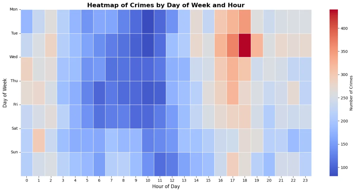
Time carried a clear signal. Incidents rose through the late afternoon and early evening, with Tuesday around 6:00 p.m. producing the single densest cell in the week. Weekdays followed a rough U-shape, quiet in the early morning and spiking from mid-afternoon into evening, while weekend activity spread out more evenly, with some early-Saturday-morning increases.
For geography I used Folium heatmaps together with KMeans clustering. Sampling 2,000 latitude/longitude points and grouping them into five clusters revealed distinct hotspots: the densest concentration sits in the downtown core, consistent with population density, foot traffic, and nightlife, with additional clusters extending into the northeast and southeast. Outer areas showed markedly fewer incidents. The clean separation between clusters confirmed that location is a strong driver of crime type and that spatial features would earn their place in the models.

Identifying the Most Important Features
To understand what actually separates violent from property crime, I trained Random Forest and XGBoost classifiers on a focused predictor set (ward, district, PSA, shift, method, hour, and day of week) with categorical fields one-hot encoded.
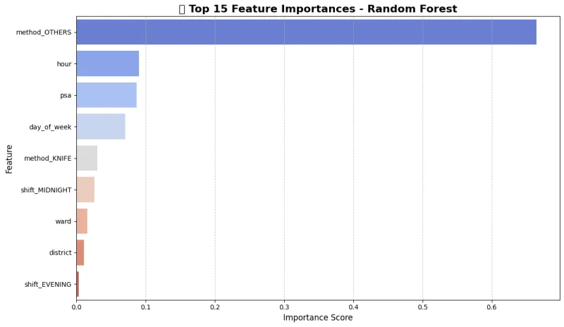
One feature dominated. method_OTHERS alone accounted for roughly 66.5% of the Random Forest importance, which makes sense: when the recorded method falls into a non-specific or uncommon category, that itself is a strong signal about the kind of incident. Beyond it, the meaningful predictors were:
- Hour of the incident
- Police Service Area (PSA)
- Day of the week
- Knife involvement
- Midnight shift
- Ward and district
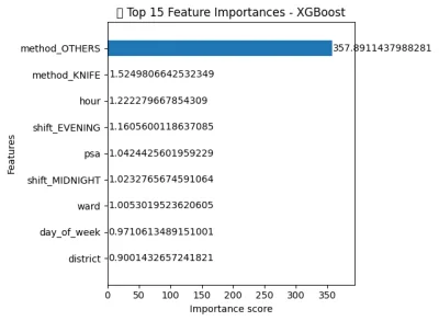
XGBoost, which ranks features by gain rather than impurity reduction, produced a nearly identical ordering, again placing method_OTHERS, hour, PSA, and day of week at the top. That agreement between two different algorithms was reassuring: behavioral and temporal information carried more predictive weight than broad administrative boundaries alone.
Comparing Traditional Machine Learning Models
I then trained five classifiers on the features method, shift, hour, day of week, and PSA. The data was split with stratified sampling into 60% training, 20% validation, and a fully untouched 20% test set (roughly 20,800 / 6,920 / 6,920 rows) so class balance was preserved everywhere and the test set stayed sealed until the very end.
Here is where headline accuracy became misleading. The validation set contained 5,845 property and 1,075 violent incidents; the models were strong on property crime and, at first glance, on accuracy, but every one of them left roughly a quarter of violent crimes undetected:
| Model | Accuracy | Violent precision | Violent recall | Violent F1 |
|---|---|---|---|---|
| Logistic Regression | 95.36% | 96.66% | 72.65% | 82.95% |
| MLP (baseline) | 95.36% | 96.66% | 72.65% | 82.95% |
| Gradient Boosting | 95.32% | 96.65% | 72.37% | 82.77% |
| XGBoost | 95.17% | 95.91% | 72.00% | 82.25% |
| Random Forest | 93.55% | 83.64% | 72.74% | 77.81% |
Validation set: 6,920 incidents (5,845 property, 1,075 violent).
The pattern is consistent: about 96 to 97% precision on violent crime but recall stuck near 72 to 73%. In plain terms, when these models flagged a crime as violent they were usually right, but they still missed more than one in four actual violent incidents. Because violent crime is the minority class and the costly one to miss, recall became the objective that mattered for the rest of the project.
Improving Minority-Class Detection
My first improvement was a deeper MLP pipeline that combined a custom frequency encoder, feature scaling, SMOTE oversampling, PCA, L2 regularization, and early stopping. This lifted violent-crime recall from about 73% to 91% while holding overall validation accuracy around 97%, with violent-class precision near 87% and a macro-F1 of 0.94. On the validation set it correctly caught 983 of 1,079 violent cases (96 missed), at the cost of 142 property cases flagged as violent, and training stopped after 56 epochs with training and validation loss tracking closely, a sign of healthy generalization rather than memorization.

I then built a custom residual neural network in PyTorch, trained on Apple’s MPS GPU backend. The architecture used two blocks of fully connected layers with skip connections, batch normalization, dropout, a classification head, the AdamW optimizer, a dynamic learning-rate scheduler, and weighted cross-entropy loss. Three deliberate imbalance strategies stacked together: engineered night/weekend-night flags to capture the temporal signature of violent crime, BorderlineSMOTE to synthesize examples near the decision boundary (yielding a balanced 35,416-sample training set), PCA down to 11 components while retaining 90% of variance, and a class weight of 2.5× on violent errors versus property errors.
Trained on 20,943 rows and validated on 6,982, the residual model reached its strongest results yet:
| Metric (violent class) | Score |
|---|---|
| Validation accuracy | 97.0% |
| Precision | 86.62% |
| Recall | 95.37% |
| F1 score | 90.78% |
| ROC-AUC | 0.995 |
Out of 1,079 violent incidents in the validation set, the residual model correctly identified 1,029 and missed only 50, with 159 property crimes flagged as violent. Validation accuracy climbed past 90% by epoch 10, crossed 96% by epoch 40, and peaked at 97.44% around epoch 59 before early stopping, and training and validation loss stayed aligned throughout, and the precision-recall curve held high precision across the recall range. Compared with the traditional models, that is a jump from ~73% to ~95% violent recall without giving up overall accuracy.
Optimizing the Decision Threshold
A binary classifier defaults to a 0.5 probability cutoff, which quietly assumes a false positive and a false negative cost the same. In public safety they don’t: missing a violent incident is far worse than over-flagging a property one. So I swept the full range of thresholds and scored each with a custom weighted metric that penalized false negatives at twice the weight of false positives.
Three thresholds stood out, each representing a different operating philosophy:
| Threshold | Precision | Recall | F1 | Role |
|---|---|---|---|---|
| 0.932 | 98.06% | 93.88% | n/a | Best weighted score (0.9811), deployed choice |
| 0.962 | 98.63% | 93.42% | 95.95% | Highest F1 and accuracy (98.78%) |
| 0.033 | 63.01% | >98% | n/a | Max-recall triage only; too many false alarms |
I selected the weighted-optimal threshold of 0.932, which best reflected the priority of catching violent incidents while keeping false alarms manageable. Relative to the default cutoff, this setting produced a 32% reduction in missed violent cases and an 87% reduction in false violent classifications. The max-recall option (0.033) captured nearly every violent crime but collapsed precision to 63%, making it viable only for a triage or surveillance queue, not for direct decisions. I wrapped the chosen threshold in a small utility so the same risk-aware cutoff carries into any downstream use, a reminder that deployment is about more than picking the highest-accuracy algorithm; the threshold has to encode the real cost of each error.
Regression and Risk-Mapping Extension
To round the project out, I reframed the same data as a regression problem aimed at strategic planning rather than case-level classification. Two targets: predicted crime counts and predicted violent-crime ratios across combinations of ward, hour, and day, with crime density normalized per capita by ward.
This extension compares seven regressors (Random Forest, Gradient Boosting, XGBoost, LightGBM, Ridge, Lasso, and ElasticNet), evaluated with R², RMSE, MAE, and explained variance. The predictions feed into composite risk scores rendered as ward-and-hour heatmaps, the kind of output that could support resource allocation and patrol planning. This section is a designed prototype layered on the classification core rather than a fully tuned model.
Final Takeaway
The biggest lesson was that strong overall accuracy can hide poor minority-class performance. The traditional models looked successful at 95% accuracy, until their ~73% violent recall exposed that they were missing a quarter of the incidents that matter most.
Through feature engineering, class balancing, cost-sensitive learning, residual deep learning, and threshold optimization, I moved violent-crime recall from about 73% to roughly 95% while holding overall accuracy near 97% and reaching a 0.995 ROC-AUC, identifying far more violent incidents without sacrificing performance on the majority class.
The end result is a complete data science workflow spanning data cleaning, spatial analysis, supervised and unsupervised learning, deep neural network development, model interpretation, and risk-aware evaluation. It is meant as an analytical research prototype, not a replacement for human judgment or a standalone policing decision system.
Data and Code
- Notebook (all code and outputs): DC Crime Analysis on Kaggle
- Source data: Crime Incidents in 2024 and Crime Incidents in 2023, published by the DC Metropolitan Police Department on Open Data DC

0 comments
Sign in to comment. No password, and nothing is posted anywhere on your behalf. We receive your name and email from the provider, nothing else. See privacy and the comment rules.
More about signing in